Although the linear regression model is simple and used frequently it's not adequate for some purposes. For example, imagine the response variable y to be a probability that takes on values between 0 and 1. A linear model has no bounds on what values the response variable can take, and hence y can take on arbitrary large or small values. However, it is desirable to bound the response to values between 0 and 1. For this we would need something more powerful than linear regression.
Another problem with the linear regression model is the assumption that the response y has a constant variance. This can not be the case if y follows for example a binomial distribution (y ~ Bin(p,n)). If y also is normalized so that it takes values between 0 and 1, hence y = Bin(p,n)/n, then the variance would then be Var(y) = p*(1-p), which takes on values between 0 and 0.25. To then make an assumption that y would have a constant variance is not feasible.
In situations like this, when our response variable follows a binomial distribution, we need to use general linear regression. A special case of general linear regression is logistic regression, which assumes that the response variable follows the logit-function shown in Figure 4.
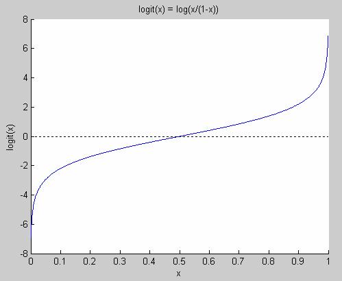
Figure 4 The logit function
Note that it's only defined for values between 0 and 1. The logit function goes from minus infinity to plus infinity. The logit function has the nice property that logit(p) = -logit(1-p) and its inverse is defined for values from minus infinity to plus infinity, and it only takes on values between 0 and 1.
However, to get a better understanding for what the logit-function is we will now introduce the notation of odds. The odds of an event that occurs with probability P is defined as
odds = P / (1-P).
Figure 5 shows how the odds-function looks like. As we can see, the odds for an event is not bounded and goes from 0 to infinity when the probability for that event goes from 0 to 1.
However, it's not always very intuitive to think about odds. Even worse, odds are quite unappealing to work with due to its asymmetry. When we work with probability we have that if the probability for yes is p, then the probability for no is 1-p. However, for odds, there exists no such nice relationship.
To take an example: If a Boolean variable is true with probability 0.9 and false with probability 0.1, we have that the odds for the variable to be true is 0.9/0.1 = 9 while the odds for being false is 0.1/0.9 = 1/9 = 0.1111… . This is a quite unappealing relationship. However, if we take the logarithm of the odds, when we would have log(9) for true and log(1/9) = -log(9) for false.
Hence, we have a very nice symmetry for log(odds(p)). This function is called the logit-function.
logit(p) = log(odds(p)) = log(p/(1-p))
As we can see, it is true in general that logit(1-p)=-logit(p).
logit(1-p) = log((1-p)/p) = – log(p/(1-p)) = -logit(p)
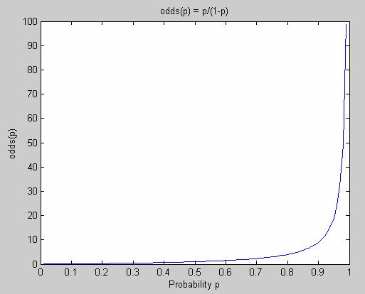
Figure 5 The odds function
The odds function maps probabilities (between 0 and 1) to values between 0 and infinity.
The logit-function has all the properties we wanted but did not have when we previously tried to use linear regression for a problem where the response variable followed a binomial distribution. If we instead use the logit-function we will have p bounded to values between 0 and 1 and we will still have a linear expression for our input variable x
logit(p) = a + ![]() * x.
* x.
If we would like to rewrite this expression to get a function for the probability p it would look like

No comments:
Post a Comment